Practical Examples
Computer Activity Dataset (Regression)
Computer Activity dataset describes the portion of time that CPUs run in user-mode, based on 8192 computer system activities collected from a Sun SPARCstation 20/712 with 2 CPUs and 128 MB of memory running in a multi-user university department, and each system activity is evaluated using 12 system measures (number of reads and number of writes between system memory and user memory, number of system calls of all types, number of system read calls, number of system write calls, number of system fork calls, number of system exec calls, number of characters transferred by read calls, number of characters transferred by write calls, process run queue size, number of memory pages available to user processes, and number of disk blocks available for page swapping).
Number of Attributes: 12
Number of Instances: 8,192
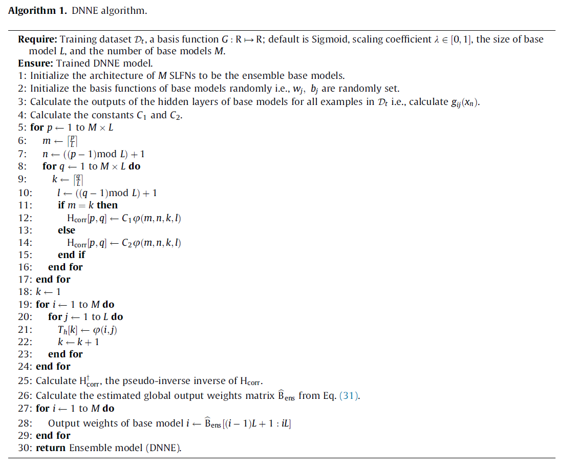
 The approximated function
clear all;
data = csvread('data/computer_activity.data');
X = data(:,
2:end);
T = data(:, 1);
dnne = newdnne(5,
70, X, T, 0.5);
[dnne, rmse] = traindnne(dnne, X, T);
netOut = simdnne(dnne,
X);
rmse1 = sqrt(sum((T
- netOut).^2) / size(T,1));
Calfornia Housing Dataset (Regression)
California Housing dataset contains 20,640 observations for estimating the median house prices in California, U.S. Each characterized by eight continuous features (median income, housing median age, total rooms, total bedrooms, population, households, latitude, and longitude).
Number of Attributes: 8
Number of Instances: 20,640
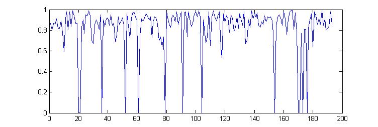
 The approximated function
clear all;
data = csvread('data/calhousing.data');
X = data(:,
2:end);
T = data(:, 1);
dnne = newdnne(5,
50, X, T, 0.55);
[dnne, rmse] = traindnne(dnne, X, T);
netOut = simdnne(dnne,
X);
rmse1 = sqrt(sum((T
- netOut).^2) / size(T,1));
German Credit Dataset (Binary Classification)
Number of Attributes: 24
Number of Instances: 1,000
Number of Classes: 2
clear all;
data = csvread('data/credit_german.data');
X = data(:,
2:end);
TOrig = data(:,
1);
noClasses = max(TOrig);
T = ones(size(TOrig,1),
noClasses) * -1;
for i=1:noClasses
T(TOrig
== i, i) = 1;
end
clear noClasses data i;
dnne = newdnne(5,
100, X, T, 0.55);
[dnne, rmse] = traindnne(dnne, X, T);
predLabels = simdnne(dnne,
X, 'class');
acc = sum(TOrig ==
predLabels) / size(TOrig,1) * 100;
Led-7 Dataset (Multi-class Classification)
This simple domain contains 7 Boolean attributes and 10 concepts,
the set of decimal digits. Recall that LED displays contain 7
light-emitting diodes and hence the reason for 7 attributes. The
problem would be easy if not for the introduction of noise. In
this case, each attribute value has the 10% probability of having
its value inverted. All attribute values are either 0 or 1, according to whether
the corresponding light is on or not for the decimal digit. Each attribute (excluding the class attribute, which is an
integer ranging between 0 and 9 inclusive) has a 10% percent
chance of being inverted.
Number of Attributes: 7
Number of Instances: 2,000
Number of Classes: 10
clear all;
data = csvread('data/led_7.data');
X = data(:,
2:end);
TOrig = data(:,
1);
if min(TOrig) == 1
noClasses
= max(TOrig);
T = ones(size(TOrig,1), noClasses) * -1;
for i=1:noClasses
T(TOrig == i, i) = 1;
end
elseif min(TOrig) == 0
noClasses
= max(TOrig) + 1;
T = ones(size(TOrig,1), noClasses) * -1;
for i=1:noClasses
T(TOrig == i - 1, i) = 1;
end
end
clear noClasses data i;
dnne = newdnne(5,
50, X, T, 0.55);
[dnne, rmse] = traindnne(dnne, X, T);
predLabels = simdnne(dnne,
X, 'class');
if min(TOrig) == 1
predLabels
= simdnne(dnne, X, 'class');
elseif min(TOrig) == 0
predLabels
= simdnne(dnne, X, 'class') - 1;
end
acc = sum(TOrig ==
predLabels) / size(TOrig,1) * 100;
Evaluation Example
In this example, we show how to evaluate the performance of a DNNE model on testing dataset that is extracted from the original dataset. This example mainly shows how to use the dnne m-function. We show this on two datasets that model regression and classification problems.
clear all;
s = RandStream('mt19937ar','Seed',1986);
for i=1:10
%
California Housing Dataset (REGRESSION)
data
= csvread('data/calhousing.data');
indexes
= randperm(s, size(data,1));
t = ceil(0.60 * size(data,1));
trainData
= data(indexes(1:t), :);
testData
= data(indexes(t+1:end), :);
[housing_dnneModel{i}, housing_trnAcc(i), housing_tstAcc(i),
housing_rmse(i)] = dnne(5, 50, 0.55, trainData,
testData, 'reg', s);
% German
Credit Card Dataset (CLASSIFICATION)
data
= csvread('data/credit_german.data');
indexes
= randperm(s, size(data,1));
t = ceil(0.60 * size(data,1));
trainData
= data(indexes(1:t), :);
testData
= data(indexes(t+1:end), :);
[credit_dnneModel{i}, credit_trnAcc(i), credit_tstAcc(i),
credit_rmse(i)] = dnne(5, 100, 0.55, trainData,
testData, 'class', s);
end
clear data trainData testData s indexes t i